Surface Detail

Articles in the On Grids series

• Let's go deeper
• Iterating on a theme
• Some useful functions
• On Grids
• Turtles all the way down

Perturbation, determinism, and line-drawing.

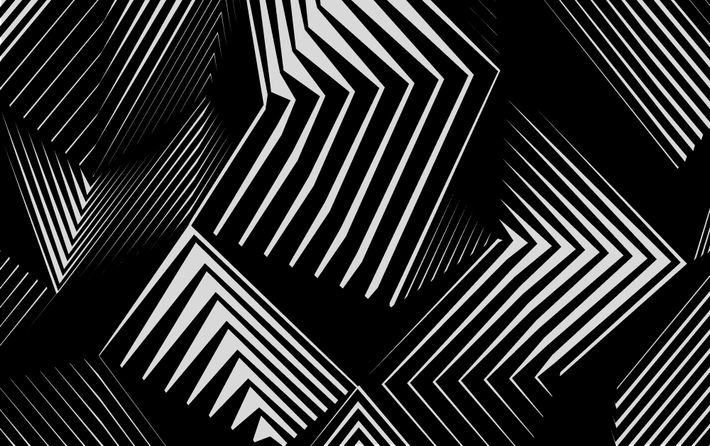
In the last post, we saw how we can break down a grid element into separate lines to introduce some seeming complexity, but that ultimately it's something of a simple structure. For reference, here's the pen we ended up with.

In this post, we're going to take on 2 tasks:

• Make the grid irregular.
• Change the width of the lines based on the edge they're coming from.

To accomplish this, we need to implement a few new concepts:

• Hashing and pseudorandomness.
• Grids with points that can be moved around.
• Lerping between two points, instead of between single numeric (scalar) values.
• Deterministic randomness (hashing) based on edge (remembering that two neighbouring cells share an edge).
• Polygons!
• Breaking a space into columns is essential to ensure the layout looks okay.

This is going to be a lot to get through, but we'll make regular check-ins along the way, and it'll all be worth it.

Hashing

Pseudorandomness and hashing are really fascinating subjects that I'll write more on at some point in the future. For our purposes, we're going to go with something very simple - a function that takes a number, regardless of how large or small, and returns a random-seeming number between zero and one.

const randomOS = Math.random() * 200;
export const hash = (x, os = randomOS) =>
  Math.abs(
    Math.sin(
      (x + os) * 9174986346
    ) * 1964286753) % 1;

That can look like a lot of nonsense to someone unfamiliar, so let me break it down a bit. This sort of hashing function takes a simple sine wave and ramps it up to an extremely large frequency (that * 917...). Then, it is multiplied by a huge amplitude and takes the fractional value of that resulting number. Given sufficiently large numbers for the frequency and amplitude values, it compresses the wave to a point where the numbers from the function appear random, but are deterministic.

In the above codepen, you can play around with this function directly by moving a point along the sinewave to see the values it outputs. But as a further demonstration, take a look at the following code.

hash(1); // 0.09126
hash(2); // 0.11871
hash(3); // 0.60281
hash(3); // 0.60281
hash(3); // 0.60281

Grid perturbation

Lerping points

This is where things start to get exciting. All we really mean by perturbation is that the points can be moved around, making the grid cells irregularly shaped.

Like lerp, lerpPoint takes two values representing the beginning and the end of a ratio, and a scalar value representing the point along the ratio to return the value.

Consider the previous code we were using to lerp between two points:

  const topEdgePoint = {
    x: lerp(
      cell.points[0].x, 
      cell.points[1].x, 
      interpolant
    ),
    y: cell.points[0].y,
  };

Notice how the only value we're lerping is the X value? This is called a "scalar" value, because it only has a single value. The official definition is that it only has magnitude, not direction.

What we need is a function that can lerp both the X and the Y values at the same time. If you'll remember our scalar lerp function, extending that into 2 dimensions is relatively trivial, see:

lerp = (a, b, t) =>
  a + (b - a) * t;
lerpPoint = (p1, p2, t) => ({
  x: lerp(p1.x, p2.x, t),
  y: lerp(p1.y, p2.y, t),
});

We need this new function because we now need to perform a lerp between two points, instead of 2 scalar values. Suddenly, with this function, we can perform lerps like this:

Moving points

Alright, here's where things start to get fun. We'll be working from this pen as a base.

The first thing we need to do is replace the old code that was using scalar lerp to determine the position along the horizontal or vertical sides. That looked something like this:

  const topEdgePoint = {
    x: lerp(
      points[0].x, 
      points[1].x, 
      e),
    y: points[0].y,
  };

Now we can replace that with our new lerpPoint function, and it turns into this:

  const topEdgePoint = lerpPoint(
    points[0], 
    points[1], 
    e + topEdge.r);

Much nicer and easier to understand, right?

Next, we need to update our points to add a bit of perturbation. This is going to involve:

• Getting the point's ID, a scalar number, based on the x and y position of the point (remembering that our points are all in grid units).
• Getting a random angle using our hash function.
• Offsetting the point using a trigonometric function.

Before we get started, let's introduce a new variable called perturbSize. This will be a number between 0 and 0.5 and will be used to describe how far along the angle the points should move.

const perturbSize = 0.3;

Alright, now in our split loop, right before we calculate the values of the side points, let's update our point generation to look like this:

  const points = cell.points.map((point) => {
    const pointID = 
          getPointID(point.x, point.y, gridW);
    const angle = 
          hash(pointID, seed) * Math.PI * 2;
    const length = 
          hash(pointID, seed+100) * perturbSize;
    return {
      x: (
        point.x + 
        Math.cos(angle) * 
        length) * cellWidth,
      y: (
        point.y + 
        Math.sin(angle) * 
        length) * cellHeight,
    }
  })

Alright, there's a lot to break down in this function, so let's explain it with a graphic.

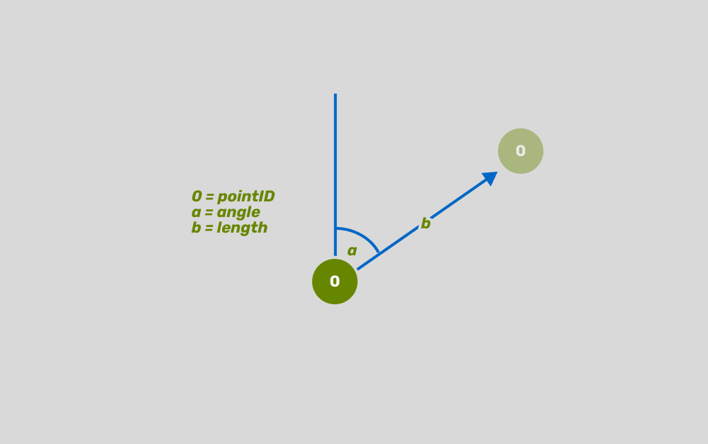
This diagram explains exactly what happens in that function. First, we get the value of the point ID (0), then we generate two pseudo-random numbers based on that ID (angle and length). The reason we're adding 100 to the seed in the second hash function is to ensure we get a different hash value for the same number.

Finally, we use these values to perform basic trigonometry to determine how far and in what direction our point moves.

You might ask why we use polar coordinates and not just generate a hash value for X and one for Y. The reason for that is distribution! Modifying the X and Y coordinates like that will move the points around in a square-like pattern, which, using polar coordinates, will move them around in a circular pattern, which can be more natural.

Take a look at this pen to see this all in action! This takes the work we did in the last post and adds to it what we've spoken about here.

What to do next

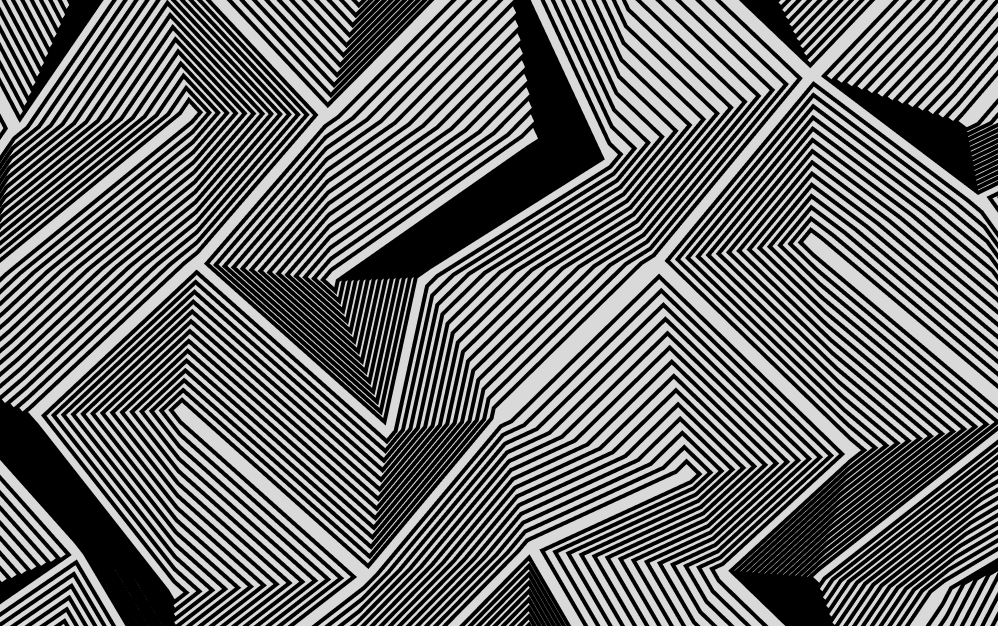
Now that we have different lines working and grid perturbation. The next thing I want to do is make it so that I can draw lines from one edge to the other edge at different widths on each edge. Something like this:

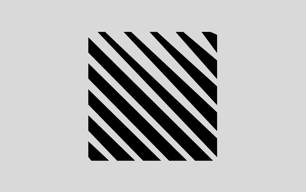
Here you can see we have those same lines running from edge to edge, but at different widths. You'll recall that we have functions to get IDs for the different edges, which will allow us to generate deterministic randomness per edge, which will provide what we need to create this.

Previously, we've only been drawing single lines from one edge to another, which has allowed us to ignore some pretty significant complexities that we'll get to shortly.

A detour

We need to take a bit of a detour next to explore a couple of things we're going to need to get in place to implement the final vision. This detour will provide us with a way to create polygons that can be filled with hatching and booleaned against each other, and will allow us to explore a way to separate a space into columns and gutters (which is essential when going from lines to polygons).

Polygons

I'm going to cheat on this one and use a piece of code written by Reinde Reinder Nijhoff. It's a class used to create and manage polygons specifically for the purposes of providing clipping and hatching. You can see the version of his class I've borrowed for this purpose and modified to work with Turtleman here. This class starts by instantiating a polygon manager, which tracks polygons drawn to it for the purpose of subtracting them from other polygons.

The relevant code in the above pen is this:

// Create a new polygon
const polygon1 = polygons.create();
const points = drawNgon(
  width/2 + Math.cos(angle) * distance,
  height/2 + Math.sin(angle) * distance,
  minSize + i/divisions*maxSize,
  sides,
  angleFollowsRotor ? angle : rotor
  );
// Draw some points to it
polygon1.addPoints(...points);
// Add some hatching.
// Parameters are angle and distance apart 
polygon1.addHatching(rotor, 5);
// Outline the polygon (draw a line)
polygon1.outline();
// Draw the polygons to the toy
polygons.draw(toy,polygon1);

We'll do a bit of a deep dive into this class some other time, but for now, we have some code that can do what we want it to - create shapes with points, and fill them with shading in the form of lines.

Columns and gutters

Now we need to come up with a way to divide a space into columns and gutters. This is necessary for our purposes because if we were to naively draw from edge-to-edge, you'd end up with a thick black line down the middle, consider:

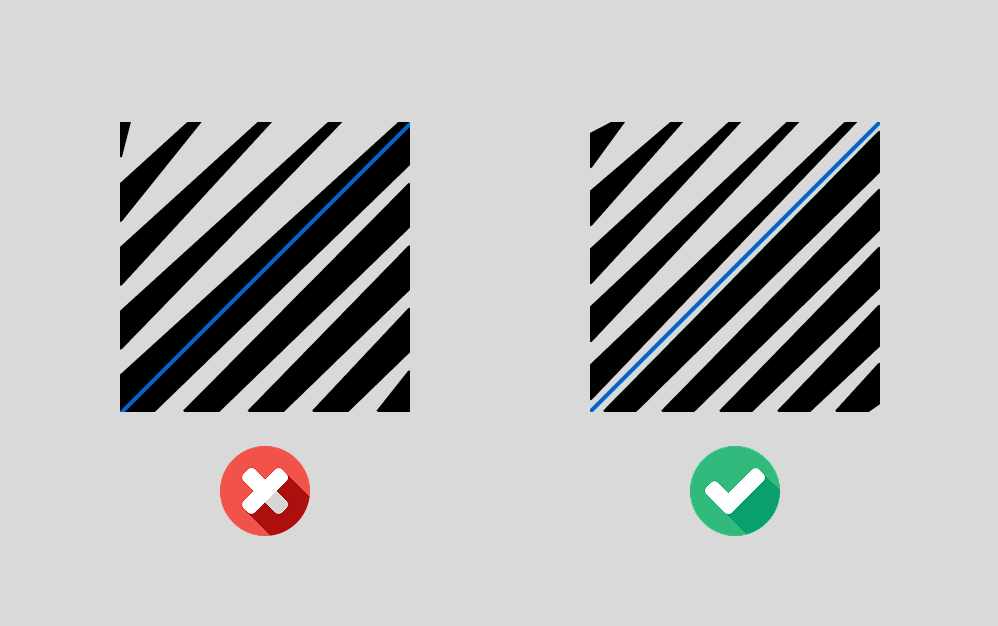
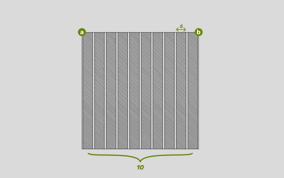
For this exercise, we should review this pen, which breaks the problem down into easy-to-understand components. The goal is to create a series of columns, each with a consistent width, separated by gutters. The size of these columns and gutters is determined by the columnSize and splits variables in our configuration. Let's break down the logic.

const columns = 10;
const columnSize = 5;
const length = a - b;
const spaceWidth = 1 / 
  ( columns * columnSize + columns ) *
  length;
const columnSizeinPx = spaceWidth * columnSize;
let x = a + spaceWidth / 2;

First, we set our total number of columns to 10 and a columnSize of 5. This columnSize isn't a pixel value; it's a ratio. It means that each column will be 5 times wider than the gutter.

The core of the logic is in the spaceWidth calculation. This variable represents the width of a single gutter. To figure this out, we treat all of our columns and gutters are proportional "units". The number of units for all columns combined is columns * columnSize, and the number of units for all gutters is simply columns. This formula implicitly adds a gutter at the start and end of the row.

Once we have the total number of units - (splits * columnSize + splits) - we can find the fractional size of a single unit by taking 1 / total_units. We then multiply that by the total available length to get our spaceWidth in pixels.

Finally, we set up the x value, which is a variable used to track the position of the "play head" as we're drawing across the area.

Drawing the polygons

Now we can use these calculated values to draw our columns. This is done inside a for loop that iterates through each split.

for (let i = 0; i < columns; i++) {
  const p = polygons.create();
  p.addPoints(
    [x, points[0][1]],
    [x + columnSizeinPx, points[0][1]],
    [x + columnSizeinPx, points[3][1]],
    [x, points[3][1]]
  );
  p.outline();
  p.addHatching(Math.PI/4,3);
  polygons.draw(toy,p)
  x += columnSizeinPx + spaceW;
}

In each iteration, we create a new polygon. The addPoints function defines the four corners of a rectangle, which becomes our column. The x variable is the key here. It starts at the correct initial position (with or without a side margin) and is then incremented at the end of each loop by the width of one column plus one gutter (columnSizeinPx + spaceW). This ensures each new polygon is placed right after the previous one, with a gutter in between.

Again, please have a play with this on codepen, it's a pretty nice little piece of code.

Bringing it all together

Now that we have the essential pieces in place—hashing, lerpPoint, point perturbation, and a way to manage polygons—we can finally combine everything to create the final effect. We’ll be taking the logic we used to create columns and gutters and applying it to each edge of our grid cells, using our hashing function to create unique, deterministic randomness for each side.

Per-edge randomness

The key to this entire effect is adapting the column layout logic to work on each of the four edges of a single grid cell. Previously, we had a single columnSize for the entire row of columns. Now, we need a unique, random size for each edge.

The following code block is where we translate the static columnSize from our previous example into a dynamic value for each edge:

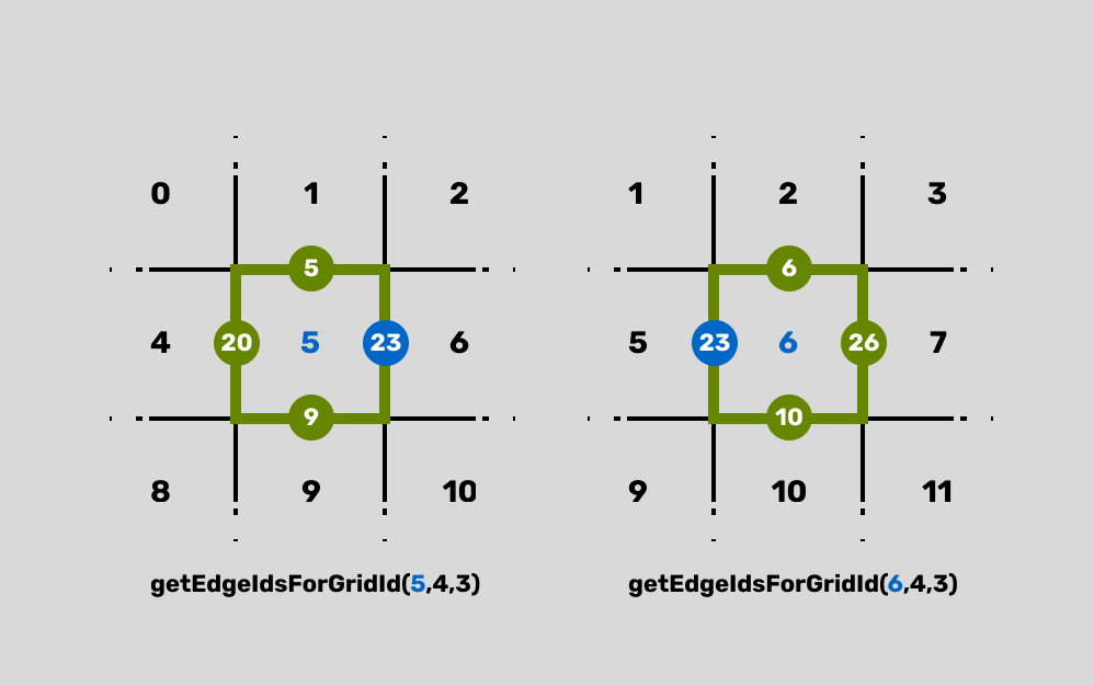
const edges = getEdgeIdsForGridId(i, gridW, gridH);
const edgeVariance = edges.map(
  (e) => hash(e, hashSeed) * sizeVariance
);
const edgeSpaces = edges.map(
  (_, i) =>
    1 / (splits * edgeVariance[i] + splits)
);
const edgeSizes = edges.map(
  (e, i) =>
    edgeSpaces[i] * edgeVariance[i]
);
const headers = edgeSpaces.map((e) => e / 2);

Let's break this down:

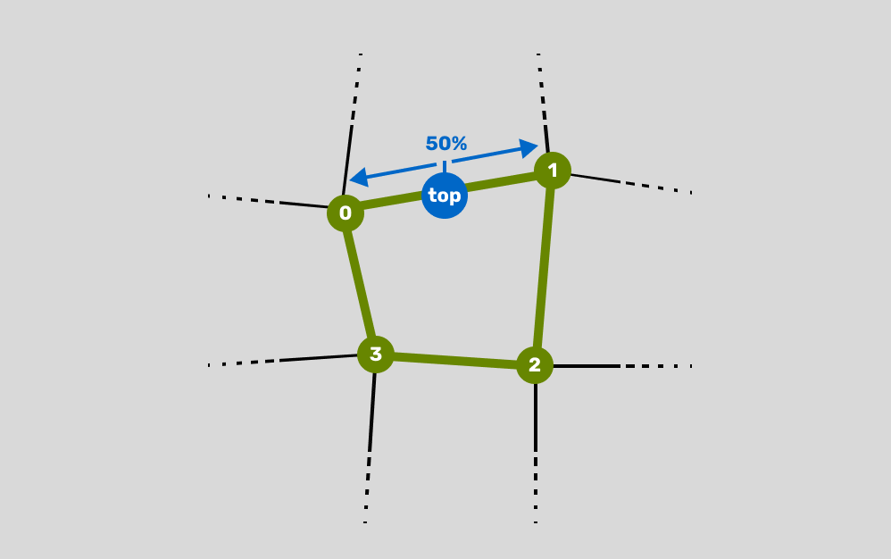
• edges: This is the function we created earlier to return an array of edge IDs for a grid cell ID. See the figure below for a further exploration of why this works.
• edgeVariance: This is where we make use of our hashing function. Remember, previously we used it to derive deterministic pseudorandom numbers for our vertices? Now we're doing the same thing for our edges. We multiply this number by the sizeVariance value from the config, which gives each edge a unique columnSize. This is what will give our lines that unique wedge shape.
• edgeSpaces: This is the exact same logic we used for our columns and gutters, but applied to each edge individually. We're calculating the width of a single gutter for each edge based on its unique edgeVariance.
• edgeSizes: This calculates the actual proportional width of the line segments on each side, just like columnSizeinPx did for our full column layout.
• headers: This is a simple array that keeps track of the marching position for our drawing loop on each edge, initialized to half of a gutter's width to account for the initial space.

Drawing the polygons

Now that we have all the necessary proportional values, we can get to the fun part: drawing the polygons. The core idea is to draw two polygons per grid cell, one connecting the top and right edges, and one connecting the bottom and left edges, or vice-versa, depending on the edgeDirection.

// ...inside the main loop
const topEdgePoints = lerpedPoints(
  points[0],
  points[1],
  headers[0],
  edgeSizes[0]
);
const leftEdgePoints = lerpedPoints(
  points[0],
  points[3],
  headers[3],
  edgeSizes[3]
);

if (edgeDirection === 1) {
  bottomEdgePoints = lerpedPoints(
    points[2],
    points[3],
    headers[2],
    edgeSizes[2]
  );
  rightEdgePoints = lerpedPoints(
    points[2],
    points[1],
    headers[1],
    edgeSizes[1]
  );
  // Draw the notches from the top edge to the right edge
  a.addPoints(
    [topEdgePoints[0].x, topEdgePoints[0].y],
    [topEdgePoints[1].x, topEdgePoints[1].y],
    [rightEdgePoints[1].x, rightEdgePoints[1].y],
    [rightEdgePoints[0].x, rightEdgePoints[0].y]
  );
  // ... and the notches from the bottom edge to the left edge
  b.addPoints(
    [leftEdgePoints[0].x, leftEdgePoints[0].y],
    [leftEdgePoints[1].x, leftEdgePoints[1].y],
    [bottomEdgePoints[1].x, bottomEdgePoints[1].y],
    [bottomEdgePoints[0].x, bottomEdgePoints[0].y]
  );
} else {
  // same logic for the other direction
}

This section of the code directly translates our previous concept of connecting lines from one edge to another into the creation of polygons. Instead of simply drawing a line, we're now defining the four points of a polygon using our lerpPoint function.

The lerpPoint function is the hero here, returning not just a single point, but a pair of points that define the width of our "line segment" on each edge. For example, topEdgePoints contains two points: one at the start of the line segment and one at the end. We then combine these pairs of points from two different edges (e.g., topEdgePoints and rightEdgePoints) to create a four-sided polygon.

This process is repeated in a loop for each of our splits, and with each iteration, we update the headers to move the drawing position forward. Finally, the code uses a boolean operation on the polygons to subtract the main polygon from the entire grid cell, leaving only the complex, hatched lines.

Play around with the code for that here - https://codepen.io/shubniggurath/pen/qEOEVMV.