Surface Detail

There's a particular quality to water. The way a single disturbance spreads outward, fades, reflects off the edges and comes back quieter than it left, the way crossing ripples interfere with each other. It feels complex. Simulating it feels like it should be difficult.

It isn't. Three numbers per point. One rule about neighbours. That's the whole thing, the rest is just iteration.

Part 1: One oscillator

Start with a single point with three properties:

• height - how far it is from its resting position
• speed - how fast it's moving
• acceleration - how hard it's being pushed

Each frame, we apply one rule: if the point is displaced from rest, pull it back. The further it's displaced, the harder the pull. This is Hooke's law. This is the same principle behind a mass on a spring, a pendulum and a plucked guitar string.

Aside: Yes math fold, while they all share the same oscillatory DNA, a pendulum actually follows F = -mg * sin(θ). For small angles, sin(θ) approx θ, which is why we can treat it as a linear spring in most simulations (certainly for this simple demonstration)!

In code, it's a single multiply:

acceleration = -elasticity * height;

That minus sign is doing all the work. If height is positive (point is above rest), acceleration is negative - it gets pushed down. If height is negative, acceleration flips positive - pushed up. The point always gets pulled back toward zero. The magnitude of elasticity controls how aggressively.

Then we just integrate - add acceleration to speed, add speed to position:

speed += acceleration;
height += speed;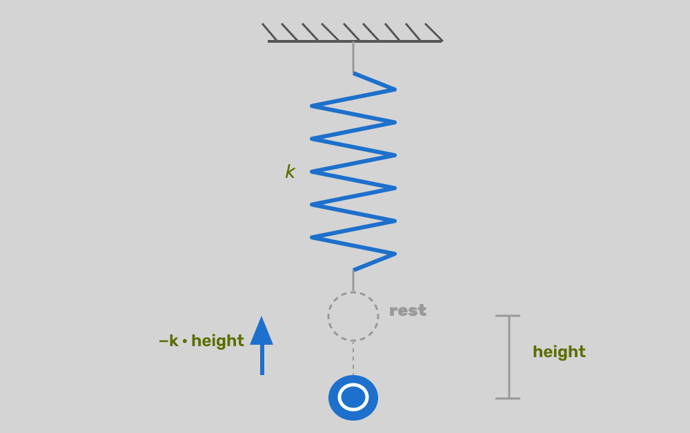

Left alone, this rings forever: the point overshoots, gets pulled back, overshoots the other way. It never settles because nothing is bleeding the energy away. Add a friction term proportional to speed and we get a result that starts to look as expected:

acceleration = -elasticity * height - friction * speed;
speed += acceleration;
height += speed;

Now every frame, a little speed is subtracted. Fast motion loses energy faster than slow motion. The oscillation decays.

Kick it, and it oscillates back to rest. That's the whole oscillator - three lines of maths.

const canvas = document.getElementById("c");
const ctx = canvas.getContext("2d");
canvas.width = window.innerWidth;
canvas.height = window.innerHeight;

// How aggressively the point is pulled back toward rest.
// Higher = snappier, faster oscillation.
const ELASTICITY = 0.004;

// How much energy is bled off per frame, proportional to current speed.
// Higher = settles quickly. Lower = rings for longer.
const FRICTION = 0.03;

const point = { height: 0, speed: 0, acceleration: 0 };

canvas.addEventListener("click", (e) => {
  // Distance from the baseline — clicking far from centre gives a bigger kick,
  // and the sign determines direction (above baseline kicks up, below kicks down).
  const distFromCentre = e.clientY - canvas.height / 2;
  point.speed = distFromCentre * 0.08;
});

function loop() {
  const baseline = canvas.height / 2;

  ctx.fillStyle = "#0f0f14";
  ctx.fillRect(0, 0, canvas.width, canvas.height);

  // Hooke's law + damping:  a = -k·x - c·v
  // The first term pulls the point back toward zero.
  // The second term resists motion — the faster it moves, the more drag.
  point.acceleration = -ELASTICITY * point.height - FRICTION * point.speed;
  point.speed += point.acceleration;
  point.height += point.speed;

  ctx.fillStyle = "#5b8dee";
  ctx.beginPath();
  ctx.arc(canvas.width / 2, baseline + point.height, 10, 0, Math.PI * 2);
  ctx.fill();

  requestAnimationFrame(loop);
}

loop();

This is a linear spring, using a basic, linear implementation of Hooke's law.

This is the only concept in the post that requires any real thought. Everything from here is just asking: what if there were more of these? What if they could see each other?

The two constants - elasticity and friction - control the character of the motion. High elasticity, low friction: fast, ringing. Low elasticity, high friction: slow, sluggish. Most of the aesthetic tuning in the final surface comes down to these two numbers.

Part 2: Two oscillators

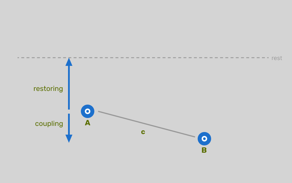
Now put two points side by side. They have their own heights and speeds, but we're going to let them talk to each other.

The rule: each point is attracted not just toward zero, but toward its neighbour's position. If the neighbour is above, it pulls up. If it's below, it pulls down. The strength of that pull is the coupling:

acceleration =
  -elasticity * height +
  (neighbourHeight - height) * coupling -
  friction * speed;

Kick one point, and watch the other respond. Energy transfers across the gap. The displaced point pulls its neighbour toward it; the neighbour resists and eventually pulls back. They trade energy back and forth, both gradually settling.

This is the core mechanism. Everything that follows is this rule, repeated.

Part 3: The chain

Extend to N points. Each one follows the same rule, now applied on both sides:

acceleration =
  -elasticity * height +
  (leftHeight - height) * coupling +
  (rightHeight - height) * coupling -
  friction * speed;

Make sure to open the control panel and increase the number of oscillators. Click here to view the full code, you can see that it’s not a significant amount more than the original example.

A few things to notice as you play with it:

Propagation speed isn't fixed; instead, it depends on the ratio of coupling strength to the implicit mass of each point (which here is 1). Higher coupling, faster, wider wave.

Reflections happen at the ends because the boundary points have no second neighbour to pull from. The wave hits the wall and bounces back in phase. This reflection is a free side effect of how the algorithm works.

Second-neighbour coupling might be worth adding, depending on your requirements. If each point also looks two steps away - at half the coupling strength - the wave shape smooths out considerably. It's a small change that makes a visible difference:

acceleration =
  -elasticity * height +
  (left1Height - height) * coupling +
  (right1Height - height) * coupling +
  (left2Height - height) * (coupling / 2) +
  (right2Height - height) * (coupling / 2) -
  friction * speed;

The second-neighbour term rounds off the peaks and gives the wave a more organic shape. You can see how you might expand this out to N neighbours.

Part 4: From dots to surface

4.1 - The naive line

The physics hasn't changed. The only thing changing now is how we draw.

Instead of individual shapes, treat each point's `height` as a vertical offset at a fixed x-position. Connect them with straight lines, close the path downward, and fill it. You've got a surface.

ctx.beginPath();
ctx.moveTo(0, baseline);
points.forEach((point, i) => {
  ctx.lineTo(segWidth * i, baseline + point.height);
});
ctx.lineTo(width, baseline);
ctx.lineTo(width, height);
ctx.lineTo(0, height);
ctx.closePath();
ctx.fill();

It works. And honestly, at low N it's quite legible - you can see the individual oscillators as corners in the line. But it looks mechanical. As N increases and the segments get shorter, it starts to approach smooth, but you're paying for physics on every point. There must be a better way.

4.2 - Smoothing with beziers

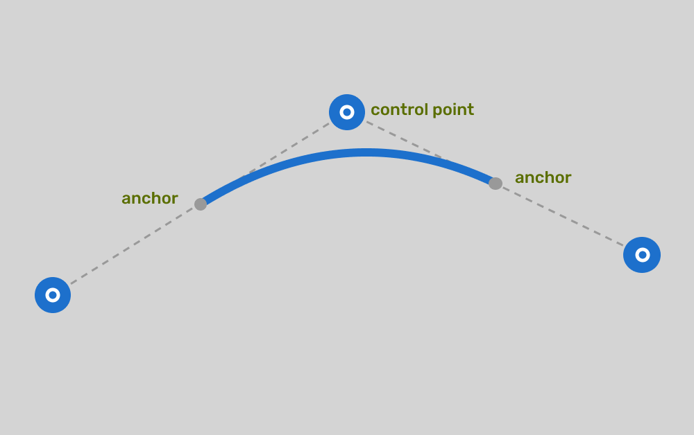
Let's smooth things out a bit. Instead of just adding additional points, we can use the points we have to draw bezier curves.

The trick: use the midpoint between each pair of adjacent points as the bezier anchor, and let the points themselves act as control points. The curve passes smoothly through every midpoint, with the shape of each segment influenced by the points on either side.

ctx.beginPath();
ctx.moveTo(0, baseline);
points.forEach((point, i) => {
  const p1 = {
    x: segWidth * (i - 1),
    y: baseline + (points[i - 1]?.height ?? 0),
  };
  const p2 = { x: segWidth * i, y: baseline + point.height };
  const xc = (p1.x + p2.x) / 2;
  const yc = (p1.y + p2.y) / 2;
  ctx.quadraticCurveTo(p1.x, p1.y, xc, yc);
});

Same physics. Same N. The surface goes from mechanical to liquid. Scroll back up to the previous demo, or click here, open the control panel and click smooth (bezier) to see the effect of this small update.

A small chain of coupled oscillators, drawn with a handful of bezier curves, looks almost like a real fluid surface, and by playing with the different oscillator properties, you can simulate different fluid types.

Part 5: Interaction

The last piece is making the surface respond to the mouse/finger in a way that feels a little more natural than clicking+dragging.

What we want is to fire a single velocity impulse when something meaningful happens: when the cursor crosses the surface.

The elegant fix is a sign-change test - ie when the direction of the cursor to the surface changes from negative to positive, or vice versa. In each frame, compare the cursor’s y-position relative to the surface midline with its position in the last frame. If the sign flips - positive to negative, or vice versa - the cursor has just crossed. Fire the impulse at that moment only:

const normalisedPos1 = mouseY - (surfaceTop + height / 2);
const normalisedPos2 = lastMouseY - (surfaceTop + height / 2);
const crossed = normalisedPos1 * normalisedPos2 < 0;

if (crossed) {
  const closestPoint = points[Math.round(mouseX / segWidth)];
  const power = clamp(deltaY * 0.02, -5, 5);
  closestPoint.speed += -power;
}

The impulse magnitude comes from deltaY - how fast the cursor was moving when it crossed. A slow drift barely disturbs the surface; a fast slash sends a big wave.

Click here to see the code in action. Cross the surface fast, cross it slow, cross it repeatedly and watch the waves stack and interfere. All of it falls out of the same three-number update rule.

Part 6: WebGPU

At a modest point count - say, 64 oscillators - the Canvas 2D approach is fine. Crank it to a couple hundred and you're running physics on every point in JavaScript, every frame, single-threaded; performance starts to become a concern.

The physics update is embarrassingly parallel. Each oscillator reads from its two neighbours and writes its own new state. No oscillator depends on what any other oscillator is doing this frame, only what they were doing last frame. That's exactly the kind of work GPUs are built for.

Moving to WebGPU means writing a compute shader that runs the physics update. One thread per oscillator. The entire chain updates simultaneously:

@compute @workgroup_size(64)
fn main(@builtin(global_invocation_id) id : vec3<u32>) {
  let i  = id.x;
  let o  = src[i];
  let lh = select(0.0, src[i - 1].height, i >= 1u);
  let rh = select(0.0, src[i + 1].height, i + 1u < uni.count);

  let accel =
    - uni.elasticity * o.height
    + ((lh - o.height) + (rh - o.height)) * uni.coupling
    - uni.friction * o.speed;

  dst[i] = Osc(o.height + (o.speed + accel * 5.0 * uni.dt) * 10.0 * uni.dt,
               o.speed  +  accel * 5.0 * uni.dt);

The trick with GPU physics is that you can't read and write the same buffer simultaneously - writing one oscillator's new state while another thread is still reading its old state gives you race conditions. The fix is ping-pong buffers: two copies of the oscillator array, src and dst. The compute shader reads src, writes dst. Next frame, swap them. The GPU never trips over itself.

With the physics running on the GPU, it's worth doing more in the render pipeline too. The vertex shader takes the key oscillators and interpolates between them using Catmull-Rom splines - smoother than quadratic beziers, and it runs entirely on GPU, so you can drive a dense mesh of render vertices from a sparse set of physics points. The fragment shader has access to the same oscillator buffer, so it can sample the surface curvature (second derivative of height) to simulate per-fragment surface normals for specular highlights.

Click here to see the code. Same physics, same three-number update rule, just a different execution model.

Part 7: The blob

So far we've been operating on the y value of each oscillator, using that to simulate waves on the surface of a body of water, but there's nothing that says we can't operate on different linear values.

Take the same chain. Instead of letting the two end points sit without a second neighbour, connect them to each other. Oscillator 0's left neighbour becomes oscillator N-1. Oscillator N-1's right neighbour becomes oscillator 0. One line of change in the compute shader:

let lh = src[(i + uni.count - 1u) % uni.count].height;
let rh = src[(i + 1u)             % uni.count].height;

This just loops the waves around the chain.

Now change what "height" means. Instead of a vertical offset from a horizontal baseline, treat each oscillator's value as a radial displacement from a base circle. Oscillator 0 sits at angle 0, oscillator 1 at angle `2π/N`, oscillator `k` at angle `k * 2π/N`. Its displacement pushes it outward or inward from the circle's edge.

The vertex shader converts that to screen coordinates using classic trigonometry:

let angle = t * TAU;
let r     = (uni.baseRadius + h) * uni.invHalf;
let x     = r * cos(angle) / uni.aspect;
let y     = r * sin(angle);

Click here to play with the code.

Conclusion

The thing I keep coming back to with simulations like this is how little causality there actually is. No point "knows" a wave is coming. No point decides to pass energy along. Each one just responds to its immediate neighbours according to a fixed local rule, and the wave emerges from that.

It's the same property that makes cellular automata interesting, or flocking algorithms, or most things in nature that look broadly coordinated from a distance. The global behaviour isn't designed. It's just what happens when simple local rules run long enough.

The surface doesn't know it's a surface, it's just a chain of springs.